[1]:
data_file = "../Simulations/toy_data_01.nc"
[2]:
import hextraj

import xarray as xr
from matplotlib import pyplot as plt
import cartopy
Load data and check raw data#
[3]:
ds_traj = xr.open_dataset(data_file)
ds_traj
[3]:
<xarray.Dataset>
Dimensions:     (traj: 144, obs: 121)
Dimensions without coordinates: traj, obs
Data variables:
    trajectory  (traj, obs) float64 ...
    time        (traj, obs) datetime64[ns] ...
    lat         (traj, obs) float32 ...
    lon         (traj, obs) float32 ...
    z           (traj, obs) float32 ...
    U           (traj, obs) float32 ...
    V           (traj, obs) float32 ...
Attributes:
    feature_type:           trajectory
    Conventions:            CF-1.6/CF-1.7
    ncei_template_version:  NCEI_NetCDF_Trajectory_Template_v2.0
    parcels_version:        2.3.1.dev20+g92f2fb90
parcels_mesh: spherical[5]:
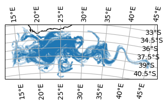
fig, ax = plt.subplots(
    1, 1,
    subplot_kw={"projection": cartopy.crs.Stereographic(
        central_latitude=ds_traj.lat.mean().data[()],
        central_longitude=ds_traj.lon.mean().data[()]
    )},
    figsize=(4, 4),
)
ds_traj.to_dataframe().plot.scatter(x="lon", y="lat", s=2, alpha=0.1, ax=ax, transform=cartopy.crs.PlateCarree())
ax.coastlines()
ax.gridlines(draw_labels=True);
Create hex labeller#
This uses a Lamber azimuthal equal-area projection which assures equal area of all hexagons and preserves angles between all vectors pointing away from the center of the projection.
We center the projection about the middle point of all trajectories.
[6]:
lon_origin = ((ds_traj.lon.max() + ds_traj.lon.min()) / 2.0).data[()]
lat_origin = ((ds_traj.lat.max() + ds_traj.lat.min()) / 2.0).data[()]
hex_size_meters = 200_000
[7]:
hex_proj = hextraj.HexProj(
    lon_origin=lon_origin,
    lat_origin=lat_origin,
    hex_size_meters=hex_size_meters,
)

hex_proj
/srv/conda/envs/notebook/lib/python3.10/site-packages/pyproj/crs/crs.py:141: FutureWarning: '+init=<authority>:<code>' syntax is deprecated. '<authority>:<code>' is the preferred initialization method. When making the change, be mindful of axis order changes: https://pyproj4.github.io/pyproj/stable/gotchas.html#axis-order-changes-in-proj-6
  in_crs_string = _prepare_from_proj_string(in_crs_string)
[7]:
HexProj(projection_name='laea', lon_origin=29.791340827941895, lat_origin=-38.089969635009766, hex_size_meters=200000, hex_orientation='flat', )
Compute labels#
Labels are three element tuples.
[8]:
ds_traj["hex_labels"] = xr.apply_ufunc(
    hex_proj.lon_lat_to_hex_AoS,
    ds_traj.lon,
    ds_traj.lat,
)

display(ds_traj)
<xarray.Dataset>
Dimensions:     (traj: 144, obs: 121)
Dimensions without coordinates: traj, obs
Data variables:
    trajectory  (traj, obs) float64 0.0 0.0 0.0 0.0 ... 143.0 143.0 143.0 143.0
    time        (traj, obs) datetime64[ns] 2021-01-01T00:30:00 ... 2021-01-31...
    lat         (traj, obs) float32 -39.17 -39.02 -38.9 ... -39.19 -39.21 -39.25
    lon         (traj, obs) float32 22.5 22.55 22.61 22.66 ... 17.16 17.18 17.17
    z           (traj, obs) float32 0.0 0.0 0.0 0.0 0.0 ... 0.0 0.0 0.0 0.0 0.0
    U           (traj, obs) float32 nan 2.598e-06 ... 1.845e-07 -7.776e-07
    V           (traj, obs) float32 nan 5.796e-06 ... -1.211e-06 -2.669e-06
    hex_labels  (traj, obs) object (-2, 1, 1) (-2, 1, 1) ... (-4, 1, 3)
Attributes:
    feature_type:           trajectory
    Conventions:            CF-1.6/CF-1.7
    ncei_template_version:  NCEI_NetCDF_Trajectory_Template_v2.0
    parcels_version:        2.3.1.dev20+g92f2fb90
parcels_mesh: sphericalAggregate data into hexagons#
Create empty dataset:
[9]:
data_agg_hex = xr.Dataset()
data_agg_hex
[9]:
<xarray.Dataset>
Dimensions:  ()
Data variables:
*empty*Aggregate particle position count:
[10]:
data_agg_hex["particle_obs_count"] = (
    ds_traj.lon
    .groupby(ds_traj["hex_labels"]).count()
)
data_agg_hex["particle_obs_count"].attrs["long_name"] = "number of positions recorded"
data_agg_hex["particle_obs_count"].attrs["units"] = None
Aggregate U, V and squared velocities:
[11]:
data_agg_hex["U"] = (
    ds_traj.U
    .groupby(ds_traj["hex_labels"]).mean()
)

data_agg_hex["U2"] = (
    (ds_traj.U ** 2)
    .groupby(ds_traj["hex_labels"]).mean()
)

data_agg_hex["V"] = (
    ds_traj.V
    .groupby(ds_traj["hex_labels"]).mean()
)

data_agg_hex["V2"] = (
    (ds_traj.V ** 2)
    .groupby(ds_traj["hex_labels"]).mean()
)
Add positions of the hex labels:
[12]:
_lon, _lat = hex_proj.hex_to_lon_lat_SoA(hextraj.aux.hex_AoS_to_SoA(data_agg_hex["hex_labels"].data))

data_agg_hex = data_agg_hex.assign_coords(lon=("hex_labels", _lon))
data_agg_hex = data_agg_hex.assign_coords(lat=("hex_labels", _lat))
[13]:
data_agg_hex
[13]:
<xarray.Dataset>
Dimensions:             (hex_labels: 28)
Coordinates:
  * hex_labels          (hex_labels) object (-5, 2, 3) ... (5, -3, -2)
    lon                 (hex_labels) float64 12.48 13.18 15.59 ... 43.39 47.1
    lat                 (hex_labels) float64 -38.38 -35.34 ... -37.3 -38.38
Data variables:
    particle_obs_count  (hex_labels) int64 82 27 206 635 311 ... 67 69 26 61 36
    U                   (hex_labels) float32 -1.309e-06 -1.814e-06 ... 2.058e-06
    U2                  (hex_labels) float32 6.788e-12 8.051e-12 ... 7.148e-12
    V                   (hex_labels) float32 -6.445e-06 -5.26e-07 ... -3.678e-06
V2 (hex_labels) float32 5.543e-11 1.045e-11 ... 1.404e-11Visualize aggregated data#
[14]:
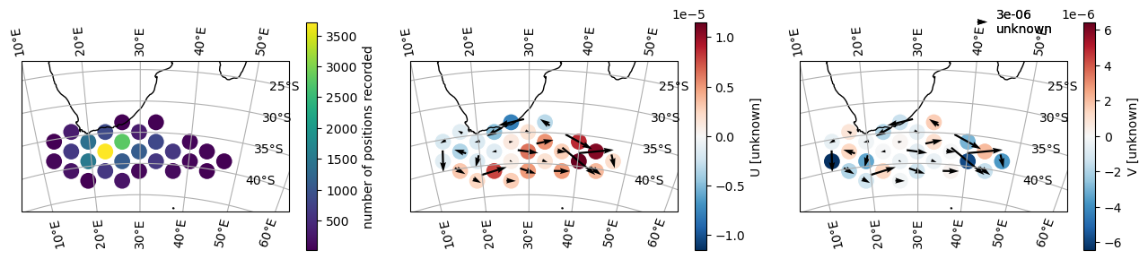
fig, ax = plt.subplots(
    1, 3,
    subplot_kw={"projection": cartopy.crs.Stereographic(
        central_latitude=lat_origin,
        central_longitude=lon_origin,
    )},
    figsize=(13, 3),
)

data_agg_hex.plot.scatter(
    x="lon", y="lat", hue="particle_obs_count", s=190,
    ax=ax[0], transform=cartopy.crs.PlateCarree(),
)

data_agg_hex.plot.scatter(
    x="lon", y="lat", hue="U", s=190,
    ax=ax[1], transform=cartopy.crs.PlateCarree(),
)
data_agg_hex.plot.quiver(
    u="U", v="V", x="lon", y="lat",
    ax=ax[1], transform=cartopy.crs.PlateCarree(),
)

data_agg_hex.plot.scatter(
    x="lon", y="lat", hue="V", s=190,
    ax=ax[2], transform=cartopy.crs.PlateCarree(),
)
data_agg_hex.plot.quiver(
    u="U", v="V", x="lon", y="lat",
    ax=ax[2], transform=cartopy.crs.PlateCarree(),
)


for _ax in ax.flat:
    _ax.coastlines()
    _ax.gridlines(draw_labels=True)
    _ax.set_extent([10, 55, -45, -22])

fig.tight_layout()
Connectivity#
[15]:
connection_count = (
    xr.merge(
        (
            ds_traj.isel(obs=0).hex_labels.rename("hex_start"),
            ds_traj.isel(obs=-1).hex_labels.rename("hex_end"),
        )
    )
    .to_dataframe().reset_index()
    .groupby(["hex_start", "hex_end"])["traj"].count()
    .rename("connection_count")
    .to_frame()
)

display(connection_count)
| connection_count | ||
|---|---|---|
| hex_start | hex_end | |
| (-2, 1, 1) | (-5, 3, 2) | 2 |
| (-4, 1, 3) | 4 | |
| (-2, 0, 2) | 2 | |
| (-2, 1, 1) | 14 | |
| (-1, -1, 2) | 3 | |
| (-1, 0, 1) | 1 | |
| (-1, 1, 0) | 5 | |
| (0, 0, 0) | 1 | |
| (1, -1, 0) | 1 | |
| (1, 0, -1) | 2 | |
| (1, 1, -2) | 1 | |
| (2, -2, 0) | 1 | |
| (2, -1, -1) | 3 | |
| (3, -1, -2) | 1 | |
| (-2, 2, 0) | (-4, 1, 3) | 4 |
| (-4, 2, 2) | 1 | |
| (-4, 3, 1) | 9 | |
| (-3, 1, 2) | 2 | |
| (-3, 2, 1) | 5 | |
| (-2, 0, 2) | 2 | |
| (-2, 1, 1) | 4 | |
| (-1, -1, 2) | 1 | |
| (-1, 0, 1) | 2 | |
| (0, -1, 1) | 1 | |
| (-1, 0, 1) | (-1, 1, 0) | 1 |
| (0, -1, 1) | 2 | |
| (0, 0, 0) | 1 | |
| (1, -1, 0) | 4 | |
| (1, 0, -1) | 3 | |
| (2, -2, 0) | 2 | |
| (2, -1, -1) | 2 | |
| (3, -1, -2) | 3 | |
| (4, -2, -2) | 1 | |
| (-1, 1, 0) | (-4, 1, 3) | 1 |
| (-3, 1, 2) | 2 | |
| (-3, 2, 1) | 2 | |
| (-2, 0, 2) | 2 | |
| (-2, 1, 1) | 13 | |
| (-2, 2, 0) | 1 | |
| (-1, 0, 1) | 1 | |
| (-1, 1, 0) | 1 | |
| (0, 0, 0) | 8 | |
| (0, 1, -1) | 2 | |
| (1, -1, 0) | 1 | |
| (1, 0, -1) | 1 | |
| (2, -2, 0) | 2 | |
| (2, -1, -1) | 5 | |
| (3, -2, -1) | 1 | |
| (4, -3, -1) | 3 | |
| (5, -3, -2) | 2 | |
| (-1, 2, -1) | (-5, 2, 3) | 1 |
| (-4, 1, 3) | 1 | |
| (-4, 3, 1) | 2 | |
| (-3, 2, 1) | 1 |
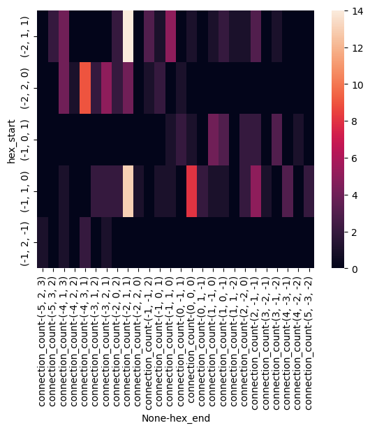
[16]:
import seaborn as sns
[17]:
sns.heatmap(connection_count.unstack(level=-1).fillna(0))
[17]:
<AxesSubplot: xlabel='None-hex_end', ylabel='hex_start'>