Gaussian Kernel Density Estimation (method 1)

One of the methods used to calculate the density of particles is a 2-dimensional horizontal Gaussian Kernel Density Estimation (GKDE). This is a non-parametric (applicable to a non-Gaussian distribution) estimate of the probability density function of a field.

In this example below, the GKDE is applied to a snapshot of particle positions, on all particles in the whole domain.

We use the python SciPy stats gaussian_kde algorithm with a default kernel size (bandwidth), which is calculated following Scott’s Rule (Scott, 1992). This bandwidth selector calculates the optimal bandwidth value that avoids both over-smoothing and under-smoothing.

• Author(s): Laura Gomez Navarro

• Created on: 11/11/22

• Last updated on:

import time

print(time.ctime(time.time()))

Sun Sep 21 18:59:56 2025

0. Imports and package versions

from glob import glob
import xarray as xr
import numpy as np
from scipy.stats import gaussian_kde

import matplotlib.pyplot as plt
import cartopy
import cartopy.crs as ccrs
from cartopy.mpl.gridliner import LONGITUDE_FORMATTER, LATITUDE_FORMATTER
import matplotlib.ticker as mticker
import inspect
import sys

1. Loading the data

filedir = '../../Simulations/'

ds = xr.open_dataset(filedir + 'toy_data_01.nc')

ds

<xarray.Dataset> Size: 627kB
Dimensions:     (traj: 144, obs: 121)
Dimensions without coordinates: traj, obs
Data variables:
    trajectory  (traj, obs) float64 139kB ...
    time        (traj, obs) datetime64[ns] 139kB ...
    lat         (traj, obs) float32 70kB ...
    lon         (traj, obs) float32 70kB ...
    z           (traj, obs) float32 70kB ...
    U           (traj, obs) float32 70kB ...
    V           (traj, obs) float32 70kB ...
Attributes:
    feature_type:           trajectory
    Conventions:            CF-1.6/CF-1.7
    ncei_template_version:  NCEI_NetCDF_Trajectory_Template_v2.0
    parcels_version:        2.3.1.dev20+g92f2fb90
    parcels_mesh:           spherical

xarray.Dataset

• Dimensions:
  • traj: 144
  • obs: 121
• Coordinates: (0)
• Data variables: (7)
  • trajectory
    (traj, obs)
    float64
    ...

    long_name :

    Unique identifier for each particle

    cf_role :

    trajectory_id

    [17424 values with dtype=float64]

  • time
    (traj, obs)
    datetime64[ns]
    ...

    long_name :

    standard_name :

    time

    axis :

    T

    [17424 values with dtype=datetime64[ns]]

  • lat
    (traj, obs)
    float32
    ...

    long_name :

    standard_name :

    latitude

    units :

    degrees_north

    axis :

    Y

    [17424 values with dtype=float32]

  • lon
    (traj, obs)
    float32
    ...

    long_name :

    standard_name :

    longitude

    units :

    degrees_east

    axis :

    X

    [17424 values with dtype=float32]

  • z
    (traj, obs)
    float32
    ...

    long_name :

    standard_name :

    depth

    units :

    m

    positive :

    down

    [17424 values with dtype=float32]

  • U
    (traj, obs)
    float32
    ...

    long_name :

    standard_name :

    U

    units :

    unknown

    [17424 values with dtype=float32]

  • V
    (traj, obs)
    float32
    ...

    long_name :

    standard_name :

    V

    units :

    unknown

    [17424 values with dtype=float32]

• Indexes: (0)
• Attributes: (5)

  feature_type :

  trajectory

  Conventions :

  CF-1.6/CF-1.7

  ncei_template_version :

  NCEI_NetCDF_Trajectory_Template_v2.0

  parcels_version :

  2.3.1.dev20+g92f2fb90

  parcels_mesh :

  spherical

2. Calculating the GKDE

2.2. Applying the GKDE functions

import numpy as np
from scipy.stats import gaussian_kde


def rem_nans(ds):
    """
    This renders lon and lat variables without nans for the last timestep.
    """
    bad_indices = np.isnan(ds["lon"][:, -1]) | np.isnan(ds["lat"][:, -1])
    good_indices = ~bad_indices
    lon_end_nonans = ds["lon"][:, -1][good_indices]
    lat_end_nonans = ds["lat"][:, -1][good_indices]

    return lon_end_nonans, lat_end_nonans


def kde_vals(lon_end_nonans, lat_end_nonans):
    """
    Calculates the KDE values and sorts x (lon) and y (lat) in function of z (KDE)

    Inputs :
    - lon_end_nonans : Longitude values free of nans
    - lat_end_nonans : Latitude values free of nans

    Outputs:
    - x : longitude values
    - y : latitude values
    - z : KDE values
    """
    x = lon_end_nonans.copy()
    y = lat_end_nonans.copy()

    xy = np.vstack([x, y])
    z = gaussian_kde(xy)(xy)

    idx = z.argsort()
    x, y, z = x[idx], y[idx], z[idx]

    return x, y, z


def kde_parcels(ds):
    """
    Inputs
    ds : xarray dataset of the parcels output netcdf file

    Outputs
    KDE for the las timestep fields of lon and lat
    """

    # Remove nans:
    lon_end_nonans, lat_end_nonans = rem_nans(ds)

    return kde_vals(lon_end_nonans, lat_end_nonans)


kde_x, kde_y, kde_z = kde_parcels(ds)

3. Plotting the outputs

3.1. Plotting cumulative distance evolution in time for the first 10 particle trajectories

fig = plt.figure(figsize=(16,17)) #(17,5)

cbar_ticks = [0.005, 0.006, 0.007, 0.008, 0.009]

ax1 = plt.subplot(111, projection=ccrs.PlateCarree())

#     ax1.set_xlim([-35.1, -18])
#     ax1.set_ylim([29.9, 40])

ss = ax1.scatter(kde_x, kde_y, c=kde_z, s=10, vmin=cbar_ticks[0], vmax=cbar_ticks[-1], cmap=plt.cm.get_cmap('viridis', len(cbar_ticks)-1), transform=ccrs.PlateCarree())
ss.cmap.set_over('r')
ss.cmap.set_under('gray')

ax1.coastlines(resolution='50m', color='black', linewidth=1, zorder=50)
ax1.add_feature(cartopy.feature.LAND, facecolor='burlywood', zorder=20)

gl = ax1.gridlines(crs=ccrs.PlateCarree(), draw_labels=True)
gl.top_labels = False
gl.right_labels = False
gl.xformatter = LONGITUDE_FORMATTER
gl.yformatter = LATITUDE_FORMATTER
gl.ylocator = mticker.FixedLocator([-42., -40., -38., -36., -34.])
gl.xlabel_style = {'size': 12}
gl.ylabel_style = {'size': 12}

cbar = plt.colorbar(ss, extend='both', orientation='horizontal')
cbar.ax.get_yaxis().labelpad = 15
cbar.ax.set_xlabel('Gaussian Kernel Density Estimation', size=14) #, rotation = 270

plt.show()

/var/folders/j5/x0w7f5sn7gg25__6pg48j82c0000gn/T/ipykernel_94936/3985650682.py:10: MatplotlibDeprecationWarning: The get_cmap function was deprecated in Matplotlib 3.7 and will be removed in 3.11. Use ``matplotlib.colormaps[name]`` or ``matplotlib.colormaps.get_cmap()`` or ``pyplot.get_cmap()`` instead.
  ss = ax1.scatter(kde_x, kde_y, c=kde_z, s=10, vmin=cbar_ticks[0], vmax=cbar_ticks[-1], cmap=plt.cm.get_cmap('viridis', len(cbar_ticks)-1), transform=ccrs.PlateCarree())

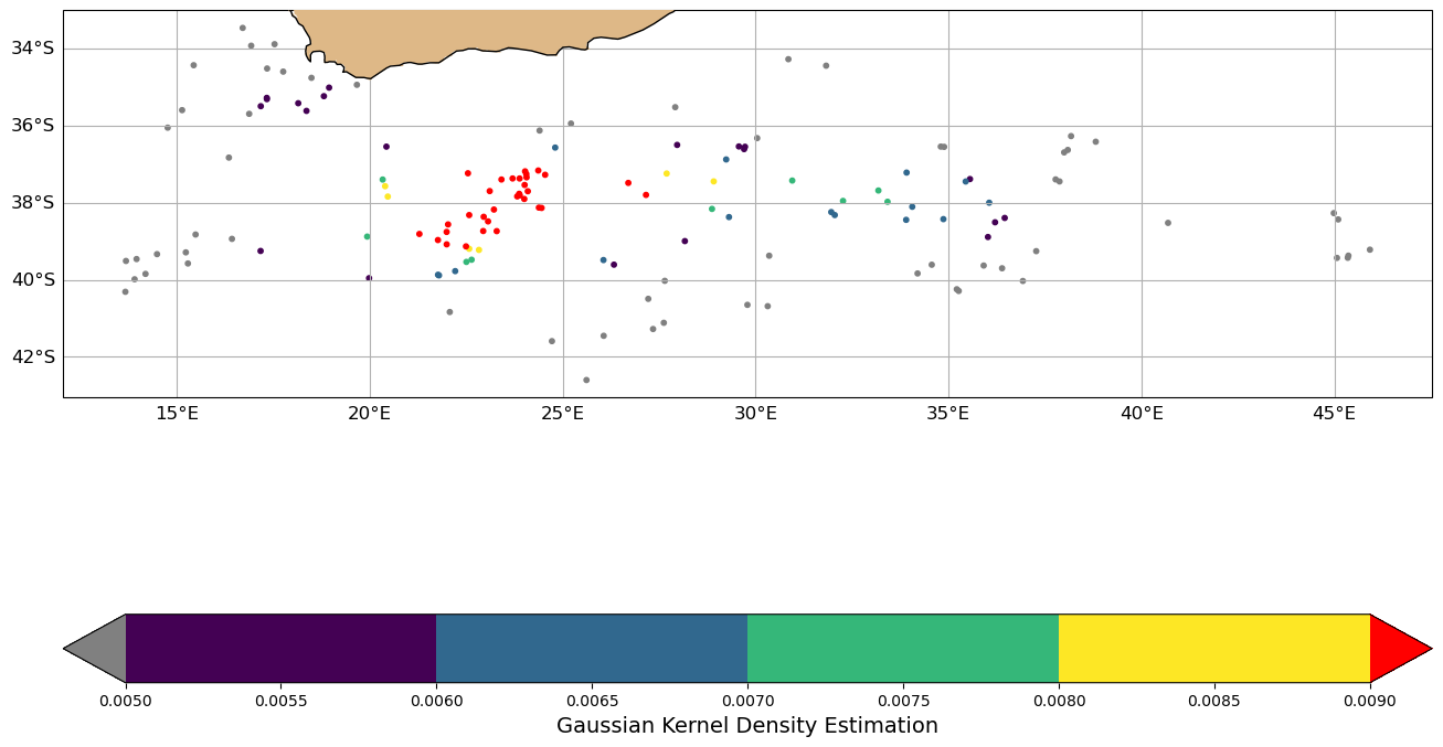
–> in this test case the GKDE does not show so clearly the accumulation zones as more particles should be released in the region of study

4. Quantification

A way to quantify then the above plot is to calculate the percentage of particles with a “high” GKDE value, that we choose it to be 0.008

• first check if any particles deleted:

ds['lon'][:,-1].values

array([26.698011, 28.164171, 27.643606, 24.718645, 37.995255, 29.234638,
       38.174526, 38.089085, 36.386173, 36.925137, 37.271023, 27.692135,
       34.057995, 33.911255, 36.052097, 27.156801, 37.874683, 25.212149,
       44.984165, 32.263596, 29.785528, 36.0202  , 33.17997 , 30.311327,
       23.818752, 25.614098, 24.09303 , 35.909134, 35.44305 , 24.450853,
       38.81421 , 31.958689, 34.563725, 33.417557, 33.89991 , 32.049088,
       21.763323, 14.18421 , 22.636242, 34.797607, 24.023075, 24.054976,
       31.82561 , 45.362434, 45.066288, 45.34612 , 35.21189 , 35.262207,
       26.059761, 15.283366, 24.001287, 22.936937, 22.500818, 24.380352,
       21.790487, 21.282694, 34.865032, 45.920753, 45.098103, 34.195713,
       22.949871, 13.661928, 27.963894, 23.287018, 23.10574 , 21.98923 ,
       24.398281, 29.69943 , 30.03786 , 28.911987, 35.554043, 36.454082,
       24.802662, 15.132946, 15.482158, 14.75911 , 22.573833, 23.885687,
       21.990768, 23.868902, 23.409975, 22.211067, 27.914537, 30.84707 ,
       27.61835 , 22.490934, 21.765697, 13.951972, 16.424952, 24.541779,
       24.06132 , 29.723223, 34.884018, 36.20441 , 37.77424 , 40.68846 ,
       18.142883, 22.070595, 24.364391, 27.339596, 27.215214, 26.326141,
       23.880114, 22.573923, 22.02631 , 29.564281, 30.349543, 29.307894,
       20.394741, 20.46407 , 23.062609, 23.215126, 19.929914, 15.229213,
       20.331572, 24.010874, 22.541416, 26.053875, 23.698732, 28.86736 ,
       16.703207, 20.428095, 14.482446, 16.92354 , 16.34547 , 15.432422,
       18.356052, 18.807606, 30.947237, 13.901372, 22.827028, 19.978989,
       19.663671, 17.329836, 17.753399, 17.171776, 16.870941, 17.327799,
       17.529312, 18.485256, 18.942495, 17.336267, 13.677705, 17.166965],
      dtype=float32)

• we calculate now the percentage of particles with a high GKDE value:

nondelp = sum(~np.isnan(ds['lon'][:,-1].data)) # calculating the total non-nan particles (none present in this
                                               # test case , but there could be some particles that values are
                                               # nan due to for example boundary conditions)

perc_high = np.round(((np.count_nonzero(kde_z >= 0.008)) / nondelp) * 100, 2)
perc_high

np.float64(26.39)