Probability Density Function**

This code bins the particle positions into histograms at each timestep using np.histogram2D. The result is a heat map of the cumulative particle density over time which, when normalised by the total number of particle positions, yields a probability map.

-Author: Jimena Medina Rubio

-Created on: 18/03/2023

0. Imports and package versions

import numpy as np
import xarray as xr
import matplotlib.pyplot as plt
import cartopy
import cartopy.crs as ccrs
import cmocean
import cmocean.cm as cmo
import pandas as pd

1. Loading the data

path="../../Simulations/toy_data_01.nc"

ds=xr.open_dataset(path)
print(ds.keys)

<bound method Mapping.keys of <xarray.Dataset> Size: 627kB
Dimensions:     (traj: 144, obs: 121)
Dimensions without coordinates: traj, obs
Data variables:
    trajectory  (traj, obs) float64 139kB ...
    time        (traj, obs) datetime64[ns] 139kB ...
    lat         (traj, obs) float32 70kB ...
    lon         (traj, obs) float32 70kB ...
    z           (traj, obs) float32 70kB ...
    U           (traj, obs) float32 70kB ...
    V           (traj, obs) float32 70kB ...
Attributes:
    feature_type:           trajectory
    Conventions:            CF-1.6/CF-1.7
    ncei_template_version:  NCEI_NetCDF_Trajectory_Template_v2.0
    parcels_version:        2.3.1.dev20+g92f2fb90
    parcels_mesh:           spherical>

2. DEFINITION OF FUNCTIONS

def probability_density(ds, bins_x, bins_y):

    """
    Calculates the PDF of the longitude and latitude coordinates of the trajectories at each observation.

    Input variables
    -ds: OceanParcels output of lon & lat of each particle at each timestep
    -bins_x & bins_y: number of bins in x/y direction
    """

    def histogram(lon, lat, bins_x, bins_y):

        #define the coordinates of the edges of the bins
        bins_edges_x = np.histogram_bin_edges(lon, bins=bins_x)
        bins_edges_y = np.histogram_bin_edges(lat, bins=bins_y)

        #calculate the 2D normalised histogram & bin edges
        H, x, y = np.histogram2d(lon.flatten(), lat.flatten(), bins=[bins_edges_x, bins_edges_y], density=True)
        return H, x, y

    #apply histogram function to all trajectories at every observation
    result = xr.apply_ufunc(
        histogram,
        ds['lon'].values,
        ds['lat'].values,
        bins_x,
        bins_y,
        input_core_dims=[['traj', 'obs'], ['traj', 'obs'], [], []],
        output_core_dims=[['binx', 'biny'], [], []],
        dask='parallelized',
        vectorize=True,
        output_dtypes=[float])

    #define the bin centres from the output bin edges
    bins_centres_x=np.linspace(result[1][0], result[1][-1], len(result[1])-1)
    bins_centres_y=np.linspace(result[2][0], result[2][-1], len(result[2])-1)

    #convert particle counts per grid cell into a data array
    da_result = xr.DataArray(result[0],
                             dims=['binx', 'biny'],
                             coords={'binx': bins_centres_x, 'biny': bins_centres_y}, name='%')

    #set values equal to zero to NaN & normalises results so that sum of probability =100
    da_result = da_result.where(da_result != 0, np.nan)*100/np.nansum(da_result)

    return da_result.T

def probability_map(probability, xlim, ylim, title, da_velocity):

    """ All-included plot of the desired domain specified by xlim & ylim """

    fig=plt.figure(figsize=(13,6))
    ax = fig.add_subplot(111, projection=ccrs.PlateCarree(central_longitude=0.0))

    #create grid
    ax.set_xlim(xlim)
    ax.set_ylim(ylim)

    #choose: plot coastlines or velocity field stored in data array
    if np.all(da_velocity is None):
        ax.coastlines(resolution='10m')
        ax.add_feature(cartopy.feature.LAND, facecolor='grey')
    else:
        da_velocity.plot(ax=ax, cmap=cmo.balance, alpha=0.7)

    gl = ax.gridlines(crs=ccrs.PlateCarree(), draw_labels=True)
    gl.right_labels = False
    gl.top_labels = False

    #plotting probability results
    probability.plot(ax=ax, cmap=cmo.matter)
    plt.title(title)

    return plt.show()

3. RESULTS

bins_x=30
bins_y=20
probability=probability_density(ds, bins_x, bins_y)

4. PLOTS

#choose the limits of the x & y axis of the graph
xlim=[10, 47]
ylim= [-47, -25]

#plot the results
probability_map(probability, xlim, ylim, 'Probability density map', None)

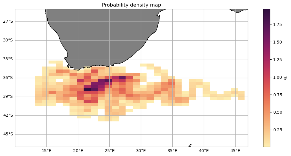
*optional: for very fine resolution regions, the original hydrodynamical data can be used to plot the pdf’s results on top so that coast is better defined in space.